How to initialize deep neural networks? Xavier and Kaiming initialization

Mar 22, 2019
deep learning paper review
17 min read

Table of Content

Initialization of neural networks isn’t something we think a lot about nowadays. It’s all hidden behind the different Deep Learning frameworks we use, like TensorFlow or PyTorch. However, it’s at the heart of why and how we can make neural networks as deep as they are today, and it was a significant bottleneck just a few years ago.

In this post, I’ll walk over the initialization part of two very significant papers:

Understanding the difficulty of training deep feedforward neural networks: the 2010 paper that introduced ‘Xavier initialization’,
Delving Deep into Rectifiers: Surpassing Human-Level Performance on ImageNet Classification: winner of the 2015 ImageNet challenge, the paper that adapted Xavier initialization into ‘Kaiming initialization’.

To ease reading, I’ll be referencing to the two papers by ‘the Xavier paper’, the ‘Kaiming paper’, sometimes even only by ‘Xavier’ and ‘Kaiming’.

First, let’s setup the problem and understand why initialization is so important.

Important note: there’s quite a bit of LaTeX formulas in this post that need JavaScript to render. It might take a bit of time to load everything properly, and obviously won’t if you deactivated JS.

The initialization headache

Why is initialization essential to deep networks? It turns out that if you do it wrong, it can lead to exploding or vanishing weights and gradients. That means that either the weights of the model explode to infinity, or they vanish to 0 (literally, because computers can’t represent infinitely accurate floating point numbers), which make training deep neural networks very challenging. And the deeper the network, the harder it becomes to keep the weights at reasonable values. We’ll see why that’s the case in the following sections.

The Xavier paper worked with neural networks with (only!) 5 hidden layers, but the effect is already very visible if no care is given to initialization.

Here’s the histogram of the mean values of the activations:

activ std init

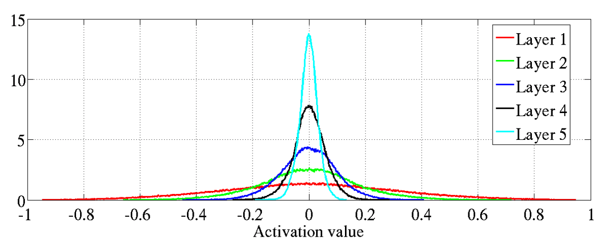
Activation values with standard initialization, source: Xavier paper

And here’s the histogram of the mean values of the backpropagated gradients:

grad std init

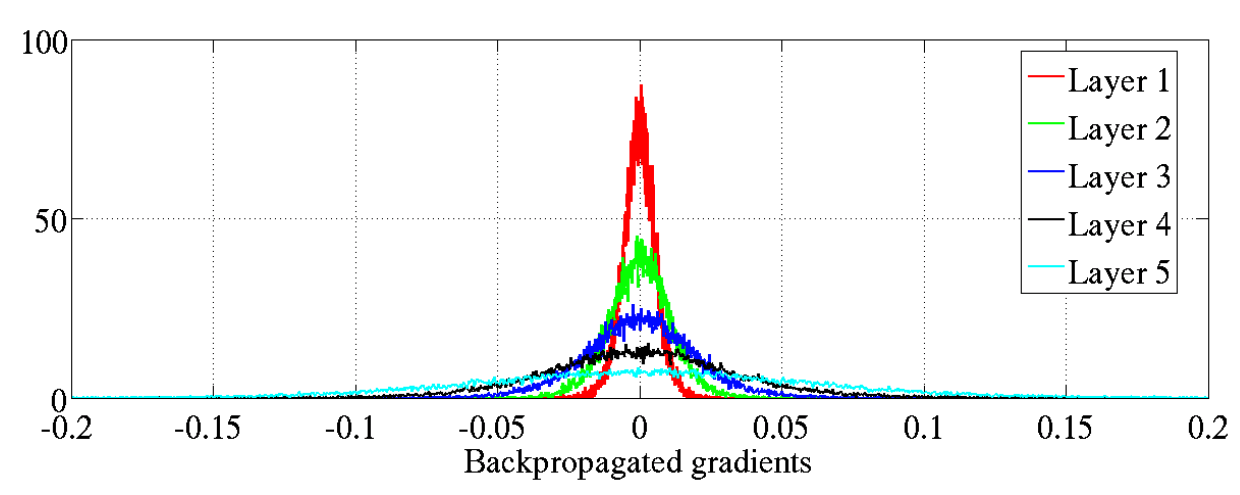
Gradient values with standard initialization, source: Xavier paper

As you can see, in this case the activation values tend to vanish, and the gradients are also vanishing (yes, vanishing, because remember they are computed backwards: from layer 5 to layer 1). And that’s only with 5 hidden layers! It’s clear we need a better way of initializing the network, that doesn’t lead to exploding or vanishing activations and gradients. That’s (one of) the contribution of Xavier initialization, that was later refined into Kaiming initialization.

Xavier and Kaiming initialization

The Xavier and Kaiming papers follow a very similar reasoning, that differs a tiny bit at the end. The only difference is that the Kaiming paper takes into account the activation function, whereas Xavier does not (or rather, Xavier approximates the derivative at 0 of the activation function by 1). Most of the math is adapted from the Kaiming paper, because I find it simpler and clearer. The main difference between this post and the papers is that this post is more detailed, so – hopefully – clearer to the uninitiated. It’s still a bit mathy though, no way around that.

Anyway, let’s get into it.

We’ll study first the forward-propagation case, then the backward one. They are quite similar but still sufficiently different that we need to do both. Then we’ll see if and how we have to take those differences into account. Finally, we’ll take a look at how better behaved deep networks become with Xavier and Kaiming initializations.

Note: when I reference an equation number, it’s clickable.

Forward-propagation

For each layer $l$, the response is written as:

$$\begin{align} \boldsymbol{y_l} = W_l \boldsymbol{x_l} + \boldsymbol{b_l} \label{eq:fwd} \end{align}$$

$\begin{align} \boldsymbol{y_l} = W_l \boldsymbol{x_l} + \boldsymbol{b_l} \label{eq:fwd} \end{align}$

Do you notice that $\boldsymbol{y_l}, \boldsymbol{x_l}$ and $\boldsymbol{b_l}$ are in bold? That means those are vectors. I know, it can be confusing. It’s to make you pay attention! Or so my teachers keep repeating to me… Anyway, here’s the definition of each term of this equation:

$\boldsymbol{x_l}$ is a $ n_l\text{-by-}1 $ vector that represents the activations of the previous layer $\boldsymbol{y_{l-1}}$ that were passed through the activation function $f$ , so we have $$\boldsymbol{x_l} = f(\boldsymbol{y_{l-1}})$$ $n_l$ is the number of activations of layer $l$ .
$W_l$ is a $d_l\text{-by-}n_l$ matrix of all the connections from layer $l-1$ to layer $l$ , with $d_l$ the number of filters of the convolutional layer (or equivalently the number of channels).
$\boldsymbol{b_l}$ is the vector of biases of layer $l$ (that are usually initialized to 0).
$\boldsymbol{y_l}$ , as mentioned before, is the vector of activations of layer $l$ before they go though the activation function.

A few hypotheses are made on those vectors:

The initialized elements in $W_l$ are mutually independent and share the same distribution.
Likewise, the elements in $\boldsymbol{x_l}$ are mutually independent and share the same distribution.
$\boldsymbol{x_l}$ and $W_l$ are independent of each other.

Under those assumptions, if we take the variance of equation $(\ref{eq:fwd})$ we get

$$\begin{align} Var[y_l] = n_l Var[w_lx_l] \label{eq:fwd_var} \end{align}$$

$\begin{align} Var[y_l] = n_l Var[w_lx_l] \label{eq:fwd_var} \end{align}$

Wait, what? Where did the bold vectors go? And what about the bias? And wasn’t that $w_l$ a bit bigger in equation $(\ref{eq:fwd})$ ? What’s $n_l$ doing here? Acute observations!

Explaining where that result comes from will take a bit of math. If you don’t speak that language (or if you are feeling confident in me, or at least in Kaiming and his co-authors), feel free to skip to equation $(\ref{eq:fwd_var2})$ , you’re not missing out on a lot.

Let $W_l = (w_{i,j})_{1 \leq i \leq d_l, \, 1 \leq j \leq n_l}$ , with all $w_{i,j}$ following the same distribution, as mentioned above. Similarly, let $\boldsymbol{x_l} = (x_j)_{1 \leq j \leq n_l}$ , with all $x_j$ following the same distribution. We have:

$$W_l\boldsymbol{x_l} = \begin{bmatrix} \sum\limits_{j=1}^{n_l} w_{1,j}x_j \\ \sum\limits_{j=1}^{n_l} w_{2,j}x_j \\ \vdots \\ \sum\limits_{j=1}^{n_l} w_{d,j}x_j \end{bmatrix}$$

$W_l\boldsymbol{x_l} = \begin{bmatrix} \sum\limits_{j=1}^{n_l} w_{1,j}x_j \\ \sum\limits_{j=1}^{n_l} w_{2,j}x_j \\ \vdots \\ \sum\limits_{j=1}^{n_l} w_{d,j}x_j \end{bmatrix}$

We then take the variance of that expression; the right handside is now equal to the trace of the variance-covariance matrix. Only the diagonal is not equal to zero: because of the independence of the variables, the covariances are null:

$$\begin{align*} Var[W_l\boldsymbol{x_l}] &= Tr \left( \quad \begin{bmatrix} Var\left[\sum\limits_{j=1}^{n_l} w_{1,j}x_j\right] & 0 & \cdots & 0\\ 0 & Var\left[\sum\limits_{j=1}^{n_l} w_{2,j}x_j\right] & \cdots & 0 \\ \vdots & & \ddots & \vdots \\ 0 & \cdots & 0 & Var\left[\sum\limits_{j=1}^{n_l} w_{d,j}x_j\right] \end{bmatrix} \quad \right) \\ \\ &= \sum_{k = 1}^{d_l} Var\left[\sum_{j=1}^{n_l} w_{k, j} x_j\right] \end{align*}$$

$\begin{align*} Var[W_l\boldsymbol{x_l}] &= Tr \left( \quad \begin{bmatrix} Var\left[\sum\limits_{j=1}^{n_l} w_{1,j}x_j\right] & 0 & \cdots & 0\\ 0 & Var\left[\sum\limits_{j=1}^{n_l} w_{2,j}x_j\right] & \cdots & 0 \\ \vdots & & \ddots & \vdots \\ 0 & \cdots & 0 & Var\left[\sum\limits_{j=1}^{n_l} w_{d,j}x_j\right] \end{bmatrix} \quad \right) \\ \\ &= \sum_{k = 1}^{d_l} Var\left[\sum_{j=1}^{n_l} w_{k, j} x_j\right] \end{align*}$

But because all the $w_{i,j}$ and the $x_i$ are independent from each other, the variance of the sum is the sum of the variances. Thus:

$$Var[W_l\boldsymbol{x_l}] = \sum_{k = 1}^{d_l} \sum_{j=1}^{n_l} Var\left[w_{k, j} x_j\right] $$

$Var[W_l\boldsymbol{x_l}] = \sum_{k = 1}^{d_l} \sum_{j=1}^{n_l} Var\left[w_{k, j} x_j\right]$

And because all the $w_{i,j}$ and $x_i$ follow the same distribution (respectively), all the variances are equal to a common variance we note $Var[w_l x_l]$ . Hence:

$$\begin{align*}Var[W_l\boldsymbol{x_l}] &= \sum_{k = 1}^{d_l} \sum_{j=1}^{n_l} Var\left[w_{l} x_l\right] \\ \\ &= d_l \times n_l \times Var\left[w_{l} x_l\right] \end{align*}$$

$\begin{align*}Var[W_l\boldsymbol{x_l}] &= \sum_{k = 1}^{d_l} \sum_{j=1}^{n_l} Var\left[w_{l} x_l\right] \\ \\ &= d_l \times n_l \times Var\left[w_{l} x_l\right] \end{align*}$

Following the exact same reasoning, albeit more simply because there’s no product, we obtain:

$$Var[\boldsymbol{y_l}] = d_l \times Var[y_l]$$

$Var[\boldsymbol{y_l}] = d_l \times Var[y_l]$

As I said, the biases are initialized to 0 thus $Var[\boldsymbol{b_l}] = 0$ . Putting it all together we obtain equation $(\ref{eq:fwd_var})$ back:

$$d_l \times Var[y_l] = d_l \times n_l \times Var[w_lx_l] \Longleftrightarrow Var[y_l] = n_l Var[w_lx_l]$$

$d_l \times Var[y_l] = d_l \times n_l \times Var[w_lx_l] \Longleftrightarrow Var[y_l] = n_l Var[w_lx_l]$

Pfiu. That was a mouthful. Let’s go on!

We now make one more assumption: that the random variable $w_l$ has zero mean. After all, setting the distribution of $w_l$ is what we’re trying to do here, so we can choose one that has zero mean. We can now further simplify equation $(\ref{eq:fwd_var})$ as follow (we also use once more the fact that $w_l$ and $x_l$ are independent):

$$\begin{align} Var[y_l] &= n_l Var[w_lx_l] \nonumber \\ \nonumber \\ &= n_l \left( \underbrace{\mathbb{E}[w_l^2]}_{=Var[w_l]} \mathbb{E}[x_l^2] - \underbrace{\mathbb{E}[w_l]^2}_{=0}\mathbb{E}[x_l]^2 \right) \nonumber \\ \nonumber \\ &= n_l Var[w_l] \mathbb{E}[x_l^2] \label{eq:fwd_var2} \end{align}$$

$\begin{align} Var[y_l] &= n_l Var[w_lx_l] \nonumber \\ \nonumber \\ &= n_l \left( \underbrace{\mathbb{E}[w_l^2]}_{=Var[w_l]} \mathbb{E}[x_l^2] - \underbrace{\mathbb{E}[w_l]^2}_{=0}\mathbb{E}[x_l]^2 \right) \nonumber \\ \nonumber \\ &= n_l Var[w_l] \mathbb{E}[x_l^2] \label{eq:fwd_var2} \end{align}$

In those formulas, $\mathbb{E}[x_l^2]$ refers to the expectation of the square of $x_l$ .

Maybe you’re asking yourself why I wrote that $\mathbb{E}[w_l^2] = Var[w_l]$ (which is true) but not $\mathbb{E}[x_l^2] = Var[x_l]$ (which is false). It’s not (only) because it allowed me to get the same result as the paper. It’s because $w_l$ has zero mean, whereas $x_l$ does not. Thus, using the expression of the variance as a function of the expectation $Var[X] = \mathbb{E}[X^2] - \mathbb{E}[X]^2$ , the square of the expectation of $w_l$ is null but not the square of the expectation of $x_l$ .

Why doesn’t $x_l$ have zero mean? That’s because it is the result of the ReLU of the previous layer ( $x_l = max(0, y_{l-1})$ ) and thus it does not have zero mean. That is also one point on which Xavier and Kaiming differ: Xavier doesn’t take into account the activation function. As a result, from here on we’ll continue with the assumption that $x_l$ is the result of a ReLU, as in the Kaiming paper, because it’s the more complex one. When we’re finished, we’ll look back to see what would have been different if we didn’t make this assumption, like Xavier, and we’ll see there’s only a small thing that needs to be modified. As a reminder, here’s the definition of the ReLU activation function:

$$ReLU(x) = \begin{cases} x \text{ if } x \geq 0 \\ 0 \text{ if } x < 0 \end{cases} = \max(x, 0)$$

$ReLU(x) = \begin{cases} x \text{ if } x \geq 0 \\ 0 \text{ if } x < 0 \end{cases} = \max(x, 0)$

Now let’s see what to do with $\mathbb{E}[x_{l}^2] = \mathbb{E}[max(0, y_{l-1})^2]$ . We assume that $w_{l-1}$ has a symmetric distribution around 0 and that $b_{l-1} = 0$ . Then $y_{l-1}$ will also have a symmetric distribution around 0, and will have zero mean. Indeed, taking the expectation of equation $(\ref{eq:fwd})$ gives us (because $w_{l-1}$ has zero mean and is independent from $x_{l-1}$ ): $$\mathbb{E}(y_{l-1}) = \mathbb{E}(w_{l-1} x_{l-1}) = \mathbb{E}(w_{l-1})\mathbb{E}(x_{l-1}) = 0$$

And because $w_{l-1}$ has zero mean and is distributed symmetrically around 0:

$$\begin{align*} \mathbb{P}(y_{l-1} > 0) &= \mathbb{P} ( w_{l-1}x_{l-1} > 0) \\ &= \mathbb{P}\left( (w_{l-1} > 0 \text{ and } x_{l-1} > 0 ) \text{ or } (w_{l-1} < 0 \text{ and } x_{l-1} < 0)\right) \\ &= \mathbb{P}(w_{l-1} >0 ) \mathbb{P}(x_{l-1} > 0) + \mathbb{P}(w_{l-1} < 0 ) \mathbb{P}(x_{l-1} < 0) \\ &= \frac{1}{2} \mathbb{P} ( x_{l-1} > 0) + \frac{1}{2} \mathbb{P} ( x_{l-1} < 0) \\ &= \frac{1}{2} \end{align*}$$

$\begin{align*} \mathbb{P}(y_{l-1} > 0) &= \mathbb{P} ( w_{l-1}x_{l-1} > 0) \\ &= \mathbb{P}\left( (w_{l-1} > 0 \text{ and } x_{l-1} > 0 ) \text{ or } (w_{l-1} < 0 \text{ and } x_{l-1} < 0)\right) \\ &= \mathbb{P}(w_{l-1} >0 ) \mathbb{P}(x_{l-1} > 0) + \mathbb{P}(w_{l-1} < 0 ) \mathbb{P}(x_{l-1} < 0) \\ &= \frac{1}{2} \mathbb{P} ( x_{l-1} > 0) + \frac{1}{2} \mathbb{P} ( x_{l-1} < 0) \\ &= \frac{1}{2} \end{align*}$

Now that we have established that $y_{l-1}$ is indeed centered on 0 and symmetric, we can compute the expectation of $x_l^2$ :

$$\begin{align*} \mathbb{E}[x_l^2] &= \mathbb{E}\left[max(0, y_{l-1})^2 \right] \\ &= \frac{1}{2} \mathbb{E}\left[y_{l-1}^2\right] \\ &= \frac{1}{2} Var[y_{l-1}] \end{align*}$$

$\begin{align*} \mathbb{E}[x_l^2] &= \mathbb{E}\left[max(0, y_{l-1})^2 \right] \\ &= \frac{1}{2} \mathbb{E}\left[y_{l-1}^2\right] \\ &= \frac{1}{2} Var[y_{l-1}] \end{align*}$

Plugging this back into equation $(\ref{eq:fwd_var2})$ , we get:

$$Var[y_l] = \frac{1}{2} n_l Var[w_l] Var[y_{l-1}]$$

$Var[y_l] = \frac{1}{2} n_l Var[w_l] Var[y_{l-1}]$

Bingo! We now have a recurrence equation between the activations at layer $l$ and the activations at layer $l-1$ . Starting from the last layer $L$ , we can thus form the following product:

$$\begin{align} Var[y_L] = Var[y_1] \left( \prod_{l=2}^{L} \frac{1}{2} n_l Var[w_l] \right) \label{eq:fwd_prod} \end{align}$$

$\begin{align} Var[y_L] = Var[y_1] \left( \prod_{l=2}^{L} \frac{1}{2} n_l Var[w_l] \right) \label{eq:fwd_prod} \end{align}$

This formula is the one that lets us see what could go wrong without a proper initialization, and thus how to design the right one. The product is key. Indeed, if we have a lot of layers (so if $L$ is large), we see that the variance of the last layer $y_L$ could be very small (if $\frac{1}{2} n_l Var[w_l]$ is below 1) or very large ( if $\frac{1}{2} n_l Var[w_l]$ is above 1). The proper value for what’s inside that product should thus be 1, and that is exactly the sufficient condition the Kaiming paper (and initialization) takes:

$$\begin{align} \forall l \,, \; \frac{1}{2} n_l Var[w_l] = 1 \label{eq:fwd_K} \end{align}$$

$\begin{align} \forall l \,, \; \frac{1}{2} n_l Var[w_l] = 1 \label{eq:fwd_K} \end{align}$

The Kaiming paper accordingly suggests to initialize the weights of layer $l$ with a zero-mean Gaussian distribution with a standard deviation of $\sqrt{\frac{2}{n_l}}$ , and null biases.

The standard deviation of the first layer isn’t that important. Indeed, looking at equation $(\ref{eq:fwd_prod})$ we can see that the variance of the first layer won’t contribute to an exponentially small or large variance at the last layer. For simplicity, we also use the same equation $(\ref{eq:fwd_K})$ to define the standard deviation of the first layer, even though to be 100% rigorous that would lead to a variance of ¹⁄₂, because there is not ReLU applied to the input.

That’s it for the Kaiming initialization in the forward case! Xavier initialization is a tiny bit different: as the activation function was assumed to be linear by Xavier (or at least approximated to be linear with a derivative of 1 around 0), it’s not taken into account, and thus the ¹⁄₂ that comes from ReLU isn’t there. The Xavier initialization formula in the forward case is hence:

$$\begin{align} \forall l \,, \; n_l Var[w_l] = 1 \label{eq:fwd_X} \end{align}$$

$\begin{align} \forall l \,, \; n_l Var[w_l] = 1 \label{eq:fwd_X} \end{align}$

Let’s tackle back-prop now!

Backward-propagation

The backward-propagation story is very similar to the forward-propagation one. The only difference is that we’re dealing with gradients, and that the flow is now from the last layers to the first ones. Accordingly, we’ll have a very similar but still slightly different result.

Instead of the forward-propagation equation $(\ref{eq:fwd})$ we had, the formula of the gradient of layer $l$ is given by:

$$\begin{align}\Delta \boldsymbol{x_l} = \hat{W}_l \Delta \boldsymbol{y_l} \label{eq:bwd} \end{align}$$

$\begin{align}\Delta \boldsymbol{x_l} = \hat{W}_l \Delta \boldsymbol{y_l} \label{eq:bwd} \end{align}$

Notice the bold symbols again. Sneaky sneaky. The terms of equation $(\ref{eq:bwd})$ are defined as follow:

$\Delta \boldsymbol{y_l}$ is the $\hat{n}_l\text{-by-}1$ gradient of the activation vector (pre-ReLU). $\hat{n}_l$ has a slightly different definition than $n_l$ , which I won’t get into. It’s not that important in the long run, just note that $\hat{n}_l \not = n_l$ because we now move through the network in the other direction.
$\hat{W}_l$ is a $c_l \text{-by-}\hat{n}_l$ weight matrix, which is just a rearrangement of $W_l$ to compute backward-propagation.
$\Delta \boldsymbol{x_l}$ is a $c_l\text{-by-}1$ vector representing the gradient of a pixel of layer $l$ .

We also make very similar assumptions to the forward-propagation case: $\hat{W}_l$ and $\Delta \boldsymbol{y_l}$ contain random variables that have the same distribution, respectively. Accordingly, we note $w_l$ and $\Delta y_l$ random variables that follow the same distribution as the ones in $\hat{W}_l$ and $\Delta \boldsymbol{y_l}$ , respectively. A hat wasn’t put on $w_l$ because $W_l$ and $\hat{W}_l$ are the same matrices, only one is rearranged from the other (so their random variables are the same). We also assume that $w_l$ and $\Delta y_l$ are independent of each other. Finally, $w_l$ has a symmetric distribution around 0 so $\Delta x_l$ has zero mean for all $l$ .

Moreover, backward-propagation involves the following equation $\Delta y_l = f'(y_l) \Delta x_{l+1}$ , where $f$ is the activation function. Convince yourself of this by writing the partial derivation of the cost function. In the case of ReLU, which we use as the active function here, here’s the derivative:

$$f'(x) = ReLU'(x) = \begin{cases} 1 \quad \text{ if } x \geq 0 \\ 0 \quad \text{ if } x < 0 \end{cases}$$

$f'(x) = ReLU'(x) = \begin{cases} 1 \quad \text{ if } x \geq 0 \\ 0 \quad \text{ if } x < 0 \end{cases}$

One last assumption: $f'(y_l)$ and $\Delta x_{l+1}$ are independent from each other. Thus, taking into account that ReLU ‘halves’ its input, at least if the input is symmetric around 0, we have:

$$\begin{align*} \mathbb{E}[\Delta y_l] &= \mathbb{E}\left( \, f'(y_l) \Delta x_{l+1}\right) \\ &=\frac{1}{2} \mathbb{E}[\Delta x_{l+1}] = 0 \end{align*}$$

$\begin{align*} \mathbb{E}[\Delta y_l] &= \mathbb{E}\left( \, f'(y_l) \Delta x_{l+1}\right) \\ &=\frac{1}{2} \mathbb{E}[\Delta x_{l+1}] = 0 \end{align*}$

and because $\Delta y_l$ has a zero mean, and that $f'(y_l)^2 = f'(y_l)$ , by taking the expectation of the square of the equation $\Delta y_l = f'(y_l) \Delta x_{l+1}$ , we get:

$$\begin{align*} \mathbb{E}\left[(\Delta y_l)^2\right] = Var[\Delta y_l] &= \mathbb{E}\left( \, f'(y_l)^2 \Delta x_{l+1} ^2 \right) \\ &= \frac{1}{2} \mathbb{E}(\Delta x_{l+1}^2) \\&= \frac{1}{2} Var[\Delta x_{l+1}] \end{align*}$$

$\begin{align*} \mathbb{E}\left[(\Delta y_l)^2\right] = Var[\Delta y_l] &= \mathbb{E}\left( \, f'(y_l)^2 \Delta x_{l+1} ^2 \right) \\ &= \frac{1}{2} \mathbb{E}(\Delta x_{l+1}^2) \\&= \frac{1}{2} Var[\Delta x_{l+1}] \end{align*}$

To remind you, we do have $\mathbb{E}(\Delta x_{l+1} ^2) = Var[\Delta x_{l+1}]$ because $\Delta x_{l+1}$ has zero mean as we just demonstrated.

We now have everything we need to compute the variance of equation $(\ref{eq:bwd})$ , with the exact same reasoning we had with the forward case (remember the big matrices?):

$$\begin{align} Var[\Delta x_l] &= Var[\hat{W}_l \Delta \boldsymbol{y_l}] \nonumber \\ &= \hat{n}_l Var[w_l] Var[\Delta y_l] \nonumber \\ &= \frac{1}{2} \hat{n}_l Var[w_l]Var[\Delta x_{l+1}] \end{align}$$

$\begin{align} Var[\Delta x_l] &= Var[\hat{W}_l \Delta \boldsymbol{y_l}] \nonumber \\ &= \hat{n}_l Var[w_l] Var[\Delta y_l] \nonumber \\ &= \frac{1}{2} \hat{n}_l Var[w_l]Var[\Delta x_{l+1}] \end{align}$

As before, we have a recurrence equation. This time it’s on $\Delta x_l$ rather than $y_l$ , but we can turn it into a product over all the $L$ layers all the same:

$$ \begin{align} Var[\Delta x_2] = Var[\Delta x_{L+1}] \left( \prod_{l=2}^{L} \frac{1}{2} \hat{n}_l Var[w_l] \right) \label{eq:bwd_prod} \end{align}$$

$\begin{align} Var[\Delta x_2] = Var[\Delta x_{L+1}] \left( \prod_{l=2}^{L} \frac{1}{2} \hat{n}_l Var[w_l] \right) \label{eq:bwd_prod} \end{align}$

Remember $x_1$ is the input of the network, that’s why the above equation “begins” at 2.

Again, as before, this product is key to understanding why the right initialization is so important: if not set carefully, the gradient can explode or vanish, depending on wether $\frac{1}{2} \hat{n}_l Var[w_l]$ is over or below 1 (strictly). Setting that number to 1 is important:

$$\begin{align} \forall l \,, \; \frac{1}{2}\hat{n}_l Var[w_l] = 1 \label{eq:bwd_K} \end{align}$$

$\begin{align} \forall l \,, \; \frac{1}{2}\hat{n}_l Var[w_l] = 1 \label{eq:bwd_K} \end{align}$

Thus we can choose a distribution with a standard deviation of $\sqrt{\frac{2}{\hat{n}_l}}$ . Lastly, same as before, the first layer wouldn’t be at the same standard deviation because no activation function is used, but the small ¹⁄₂ factor doesn’t matter because it doesn’t get compounded over $L$ layers.

The difference between this Kaiming initialization and the Xavier one is again the ¹⁄₂ that comes from the ReLU activation function. Careful, that ¹⁄₂ isn’t the one I’ve just talked about in the previous paragraph, and it’s not even coming the same way from the ReLU. The Xavier initialization in the backward-propagation case comes from the equation:

$$\begin{align} \forall l \,, \; \hat{n}_l Var[w_l] = 1 \label{eq:bwd_X} \end{align}$$

$\begin{align} \forall l \,, \; \hat{n}_l Var[w_l] = 1 \label{eq:bwd_X} \end{align}$

Yay! We figured out backward-propagation!

Bringing forward-propagation and backward-propagation together

So we have two equations very similar to each other that suggest a slightly different value for the initialization: $(\ref{eq:fwd_K})$ and $(\ref{eq:bwd_K})$ for Kaiming, and $(\ref{eq:fwd_X})$ and $(\ref{eq:bwd_X})$ for Xavier. One is the forward-propagation, the other the backward-propagation. Once again, the Xavier and the Kaiming papers take two different approaches. Xavier offers to just take the (harmonic) mean of the two (Xavier) initializations, which amounts to initializing the weights with a distribution of standard deviation of: $$\sigma = \sqrt{\frac{2}{n_l + \hat{n}_l}}$$

On the other hand, Kaiming argues that both $(\ref{eq:fwd_K})$ and $(\ref{eq:bwd_K})$ properly scale the forward and the backward signals. Indeed, if we compute the product of the quotient of $n_l$ and $\hat{n}_l$ over all $L$ layers we find a constant that only depends on the number of channels at the beginning of the network and at the end. I’m not computing that number here because I didn’t detail what $n_l$ and $\hat{n}_l$ were in terms of the other parameters of the network. If you’re interested, take a look at the end of the backward-propagation subsection in the 2.2 section of the Kaiming paper. Anyway, that number isn’t at risk of making the weights or the gradient explode or vanish, so it’s safe to just use one of $(\ref{eq:fwd_K})$ and $(\ref{eq:bwd_K})$ . No need to compute the two cases after all! Aren’t you glad I didn’t tell you this in the introduction, and I made you read the whole thing?

The results

First, let’s take a look at the contribution of Xavier initialization.

As a reminder, here’s what activations and gradients looked like with the standard initialization:

activ std init

Activation values with standard initialization, source: Xavier paper

grad std init

Gradient values with standard initialization, source: Xavier paper

And here’s what they look like with Xavier initialization:

activ Xavier init

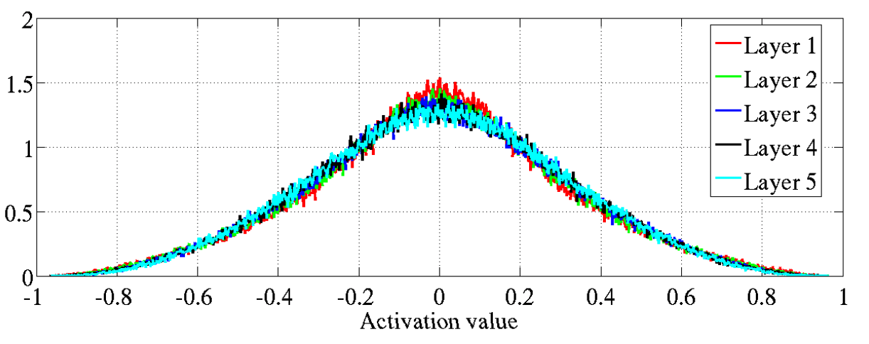
Activation values with Xavier initialization, source: Xavier paper

grad Xavier init

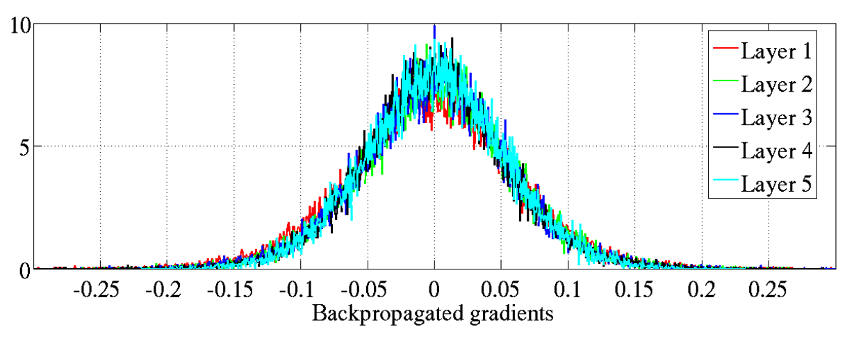
Gradient values with Xavier initialization, source: Xavier paper

That’s way better right?! Now the values don’t seem to change at all! Well, to be fair, in the activation graph layer 5 seems a tiny bit below layer 1, but hey.

As we saw, Kaiming initialization is more accurate than Xavier initialization, especially if the activation function doesn’t have a derivative of 1 at 0, like ReLU: in that case, the linear approximation of Xavier initialization is quite bad. And that badness will get compounded over all the layers so the deeper the network, the worse it’ll get.

Indeed, the Kaiming paper compares the convergence of Xavier initialization and Kaiming initialization, with a 22-layer model and with a 30-layer model, with ReLU as the activation function in both cases.

Here’s the graph for the 22-layer model:

22-layer

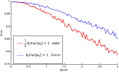
Error rate as a function of epochs with Xavier vs Kaiming initialization, 22-layer model source: Kaiming paper

In this case, Xavier initialization doesn’t fare too badly. It converges a bit more slowly than Kaiming initialization, but the Kaiming paper notes that both kinds of initialization lead to the same accuracy.

Here’s the graph for the 30-layer model:

30-layer

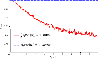
Error rate as a function of epochs with Xavier vs Kaiming initialization, 30-layer model source: Kaiming paper

In this case, Xavier initialization doesn’t even converge! This graph in particular highlights the need for Kaiming initialization if ReLU is used (and it’s kind of always used nowadays). This effect would be even worse for deep networks.

That’s it! I hope you liked my synthesis of Xavier and Kaiming initialization , and that it has helped you to understand them both.

Feel free to reach out to me on Twitter or by email if you have any question or suggestion (or if you find a typo).