
Precision, recall and the derived concepts are very important in Machine Learning (and more generally in statistics) yet can be hard to grasp. In this article I explain what they are, why they are useful and how to use them.
What’s the point ?
First off, it’s important to understand why those concepts were introduced and why they are useful. I am going to use an example throughout this post to make things clearer.
Say you have a classifier that goes through medical data and tries to figure out if someone has a particular disease or not. You’ve trained this classifier, and you want to get a good picture of exactly how good this classifier is at telling if people have the disease. Of course you can look at accuracy, the number of well-classified examples over the total number of examples. But is accuracy telling the whole picture ? Well, let’s consider those two examples:
A classifier which, if a person has the disease, will always correctly diagnose it, but gets half of the healthy people wrong. You can see that announcing to a healthy person that he or she has the disease could lead to adverse consequences.
A classifier that gets the diagnose right for every healthy person, but also miss half of the disease cases. That wouldn’t be a very good algorithm would it?
Depending on the distribution of sick to healthy patients those two classifiers could have high accuracy while not being considered very good. What’s important is that no matter if someone is sick or healthy the classifier gets it right.
Here’s a last example to see why accuracy is not enough to understand the full picture. Let’s say you are screening a population for a sickness that occurs only 1 in a 1 000 cases. Would a classifier that is 99.9% accurate seems good ? Well intuitively yes, but the classifier could just predict every person is healthy and get it right 999 out of 1000 times, so it would be 99.9% accurate. Huh. Not good.
Precision and Recall
In order to get a fuller picture of what’s going on, we need other ways to measure the performance of the classifier. To do that, let’s understand the concepts of True Positive (TP), True Negative (TN), False Positive (FP), and False Negative (FN). In all of those, the first word refers to wether the classifier got it right or not, and the second to the predicted value. For example a True Positive is when the classifier predicted a Positive and it was True. A False Negative is when an algorithm predicted a Negative but that prediction was False (it was in fact a Positive).
To say this differently, the False Somethings are the errors of the classifier, while the True Somethings are what it got right. Accordingly, there’s special names for the two types of errors a classifier can make: Type I errors for the False Positive, and Type II errors for the False Negative.
This is summed up in the following table, called a confusion matrix:
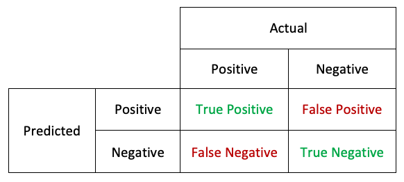
Please be sure to fully understand what those are before reading further. These concepts are essential yet can be confusing at first.
Let’s see how to compute those values in code. Suppose we have patients IDs, whether or not they have the disease, and the classifier prediction stored in a pandas DataFrame called df. The convention here is 1 to indicate the disease, 0 for no disease.
| id | disease | prediction |
|---|---|---|
| 0 | 1 | 0 |
| 1 | 1 | 1 |
| 2 | 0 | 0 |
| 3 | 1 | 1 |
| 4 | 0 | 1 |
| ... | ... | ... |
For each patient, to know wether his case is a TP, TN, FP, or FN, we need to compare the disease to the prediction. The following piece of code does that.
df.loc[(df['disease'] == 1) & (df['prediction'] == 1), 'confusion'] = 'TP'
df.loc[(df['disease'] == 1) & (df['prediction'] == 0), 'confusion'] = 'FN'
df.loc[(df['disease'] == 0) & (df['prediction'] == 0), 'confusion'] = 'TN'
df.loc[(df['disease'] == 0) & (df['prediction'] == 1), 'confusion'] = 'FP'
We now have a column called “confusion” with the confusion information.
| id | disease | prediction | confusion |
|---|---|---|---|
| 0 | 0 | 1 | FP |
| 1 | 0 | 1 | FP |
| 2 | 1 | 1 | TP |
| 3 | 0 | 0 | TN |
| 4 | 0 | 1 | FP |
| 5 | 0 | 1 | FP |
| 6 | 0 | 1 | FP |
| 7 | 0 | 1 | FP |
| 8 | 1 | 1 | TP |
| 9 | 1 | 1 | TP |
| 10 | 1 | 1 | TP |
| 11 | 0 | 0 | TN |
| ... | ... | ... | ... |
Now let’s see the definition of recall and precision.
Recall
Also called ‘Sensitivity’, recall is a measure of how well the classifier detects cases of people that do have the condition (a disease in my running example). In term of probabilities, in can be formulated as: “the probability that a sick patient is detected by the classifier”.
$$\begin{align}
recall &= \frac{True\ Positives}{True\ Positives + False\ Negatives} \nonumber \\
\nonumber \\
&= \frac{True\ Positives}{total\ number\ of\ Positives} \nonumber
\end{align}$$
So what does different values of recall mean? If $recall = 1$, that means that all patients with the disease are detected. $recall = 0.5$ would mean that only half of the patient with the disease are detected.
Let’s see how to implement that in code. Based on the dataframe we have, what we need to do is count the occurrences of 'TP' and 'FN' in the confusion column. While we’re at it, let’s do that for 'TN' and 'FP' also, we might need it later on.
TP = df[df['confusion'] == 'TN'].count()[0]
FN = df[df['confusion'] == 'FN'].count()[0]
TN = df[df['confusion'] == 'TN'].count()[0]
FP = df[df['confusion'] == 'FP'].count()[0]
We have everything to compute recall:
recall = TP / (TP + FN)
Precision
If you’ve understood everything so far the rest of this post won’t be much more complicated. However, the notions are very similar and it’s easy to forget which is which.
Precision (a.k.a. positive predicted value) is a measure of the proportion of patients thought by the classifier to have the disease that actually had the disease. In terms of probabilities it’s the following: “the probability that a patient diagnosed as sick by the classifier is sick”.
$$\begin{align}
precision &= \frac{True\ Positives}{True\ Positives + False\ Positive} \nonumber \\
\nonumber \\
&= \frac{True\ Positives}{total\ number\ of\ predicted\ Positives} \nonumber
\end{align}$$
For example, if $precision = 1$, it means that all patients diagnosed by the classifier really had the disease.
In code, with the values we calculated earlier it’s simply:
precision = TP / (TP + FP)
Specificity
Another quite useful measure is specificity. It measures how well the classifier detects a patient without the condition. It the opposite of recall : recall and specificity measures the same thing, but recall for the positives and specificity for the negatives. In terms of probabilities: “the probability that a healthy patient is diagnosed as such by the classifier”. Accordingly, the formula is very similar to that of recall: just switch the words positive and negative.
$$\begin{align}
specificity &= \frac{True\ Negatives}{True\ Negatives + False\ Positives} \nonumber \\
\nonumber \\
&= \frac{True\ Negatives}{total\ number\ of\ Negatives} \nonumber
\end{align}$$
And here’s how to compute specificity in Python.
specificity = TN / (TN + FP)
Huh.
Few, that’s quite a mouthful. If you weren’t already familiar with those concepts before it’s probably all mangled in your head right now. Don’t worry about it, it’s perfectly normal. You’ll get used to it with practice, and you’ll probably have to come back to this page or Wikipedia many times. I encourage you to play with these notions yourself. For example if you’ve built a classifier, even if you don’t need to compute precision or recall or specificity, do it in order to cement the knowledge. And it’s likely you’ll gain some valuable insight in the process!
Derived measure
The different metrics mentioned here are useful in themselves, but there are also other measures that build on the notions of precision, recall, and more generally the four confusion metrics. One of them is the $F_\beta$ score.
$F_\beta$ score
This is a bit heavier on math. You can skip the bit you don’t understand and just focus on what you get. The math-heavy stuff isn’t that useful for practical applications.
The $F_\beta$ score is a generalization of the $F_1$ score. Let’s first look at the latter. Its definition is the following:
$$\begin{align}
F_1 &= \bigg( \frac{recall^{-1} + precision^{-1}}{2} \nonumber \bigg)^{-1} \\
\nonumber \\
&= 2\cdot \frac{precision \cdot recall}{precision + recall} \nonumber
\end{align}$$
As you can see, the $F_1$ score is the weighted average of Precision and Recall. More precisely, it is the harmonic mean of precision and recall. It’s very useful to look at the $F_1$ score when you’re trying to balance the precision/recall tradeoff.
Why is the harmonic mean used instead of the classic arithmetic mean? To understand, let’s look at a classifier with a precision of 1 and a recall of 0.2. That classifier is quite poor : it detects only 20% of the sick patients. The arithmetic mean of precision and recall would be 0.6 in that case. The harmonic mean would be: $$ \frac{2 \cdot 1 \cdot \frac{2}{10}}{1 + \frac{2}{10}} = \frac{4}{12} = \frac{1}{3} $$ Indeed, 0.333… seems like a better score than 0.6.
Here’s the relevant python code.
F1 = 2 * precision * recall / (precision + recall)
However, you can be in a case when you value more the precision, or more the recall. In that case, you can use the $F_\beta$ score which is the same as the $F_1$ score but use the parameter $\beta$ to balance the importance of precision and recall.
$$ F_\beta = \frac{(\beta^2 + 1) \cdot precision \cdot recall}{\beta^2 \cdot precision + recall} \quad \text{with} \quad 0 < \beta < +\infty$$
When $\beta = 1$, the $F_\beta$ score is equal to $F_1$. If $\beta > 1$, the score puts more importance on recall, and if $\beta < 1$, the score puts more importance on precision.
How is $\beta$ defined? The exact definition is the following: $$\beta = \frac{precision}{recall} \quad \text{where} \quad \frac{\partial F_ \beta}{\partial precision} = \frac{\partial F_ \beta}{\partial recall} $$ What you need to understand from this definition is that $\beta$ is the ratio between precision and recall. The second bit shouldn’t really concern you as you are the one manually setting $\beta$ in most cases (it can be seen as an advice of how to fix $\beta$).
You might ask why is there a $\beta^2$ in the formula instead of a simple $\beta$. That comes from how the $F_ \beta$ score was built by Van Rijsbergen. At the beginning $F_ \beta$ was defined via another measure called effectiveness as $E = 1 - F_\beta$. $\beta$ was set to replace the $\alpha$ parameter in the definition of $E$, and if you do the calculation you end up with $\alpha = \frac{1}{\beta^2 + 1}$. If you’re interested in the details, see this paper that explains it well.
Fbeta = (beta**2 + 1) * precision * recall / (beta**2 * precision + recall)
I hope this article helped you to understand the confusion metrics. Feel free to reach me out on Twitter if you have any question!